User Manual for Rodin v.2.3: The First Proof

2.9.4 The First Proof

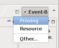
In this section, we prove the model of the Celebrity Problem. To do this, click on the box in the upper right hand corner that has a little plus sign to switch to the Proving Perspective. You can switch between perspectives using the shortcut bar as shown in Figure 2.17.

$\includegraphics{img/tutorial/tut_08_switch_perspective.png}$

Figure 2.17: Switch Perspective

$\includegraphics[width=7mm]{img/warning_64.png}$
If the Proving Perspective is not available in the menu, select Other... $\rangle$ Proving. This will open a new window which shows all available perspectives.

We should now see the window in Figure 2.18.

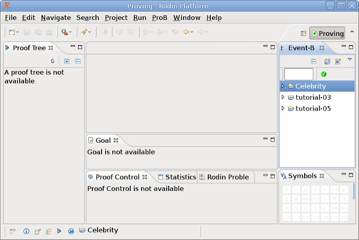
$\includegraphics{img/tutorial/tut_08_proving_perspective.png}$

Figure 2.18: Rodin Proving Perspective

The Proving Perspective contains three new important views:

Proof Tree View (3.1.5.2): Here we see a tree of the proof that we have done so far and the current position in it. By clicking in the tree, we can navigate inside the proof. Currently, we have not started with the proof, so there is no new place to move to.
Proof Control View (3.1.5.4): This is where we perform interactive proofs.
Goal View (3.1.5.3): This window shows what needs to be proved at the current position inside the proof tree.

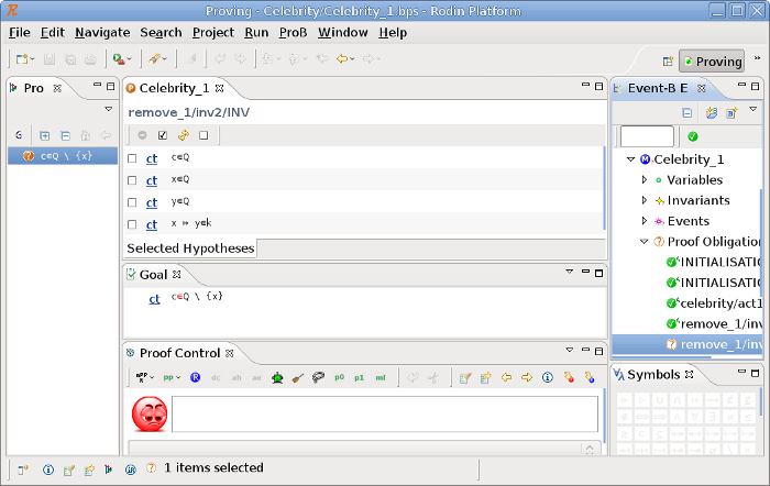
Expand the Celebrity_1 machine in the Event-B Explorer. Then expand the Proof Obligations section. We can see that the auto prover (3.1.6) did quite a good job. Only three proofs have not been completed¹ (a completed proof is indicated by a green check).

Let’s start with the proof remove_1/inv2/INV of Celebrity_1. To do this, double click on the proof obligation remove_1/inv2/INV. We should now see the window as shown in Figure 2.19.

$\includegraphics{img/tutorial/tut_08_proof2.png}$

Figure 2.19: Proof Obligation

$\includegraphics[width=7mm]{img/info_64.png}$
Make sure that you understand the different buttons in the Proof Control View (3.1.5.4).

What has to be proven is that the event remove_1 preserves the invariant inv2, $c\in Q$ . The event’s action assigns to $Q$ the new value $Q\setminus \{ x\}$ . Because we know that invariant $c\in Q$ held before the assignment, it suffices to prove that we do not remove $c$ from $Q$ , i.e. $x \neq c$ . Type this into the Proof Control View (3.1.5.4) and press the $\includegraphics[height=2ex]{img/icons/rodin/ah_prover.png}$ button.

$\includegraphics[width=7mm]{img/info_64.png}$
In order to revert a step, click on a node in the Proof Tree View and click on the $\includegraphics[height=2ex]{img/icons/rodin/pn_prover.png}$ button in the Proof Control View or open the context menu of a node and select Prune.

Take a look at the Proof Tree View. The root node should now be labeled with ah (), that is the hypothesis we just added. The node has three children: The first is the proof of well-definedness condition of $x\neq c$ which is just $\mathord {\top }$ and trivially proven. The second is the proof of the hypotheses $\lnot x=c$ . The third is the proof of the original goal where the new hypotheses can be used.

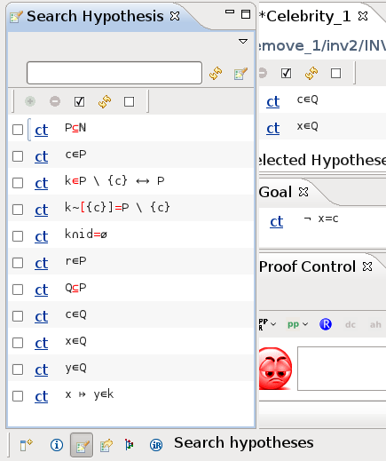
The new goal is $\lnot x = c$ . Now, try selecting the right hypotheses by yourself in order to complete the proof (Hint: What axiom states that the celebrity does not know anybody?). To do this, click on the $\includegraphics[height=2ex]{img/icons/rodin/sh_prover.png}$ button in the Proof Control View. On the left side we should see now the Selected Hypotheses View (see Figure 2.20). If you cannot find the right hypotheses, you may also just select all hypotheses. To add the selected hypothesis to the Selected Hypotheses View just click on the $\includegraphics[height=2ex]{img/icons/rodin/add.png}$ button.

$\includegraphics{img/tutorial/tut_08_search_hypothesis.png}$

Figure 2.20: Search Hypothesis View

Now click on the p0 button to prove the goal $\lnot x = c$ with the Predicate prover on selected hypothesis. The goal should be discharged and in the Proof Tree you should see that the first two children of the root node are proven. The Proof Control View should now show the original goal $c \in Q \setminus {x}$ and $x\neq c$ is now one of our hypotheses. Click a second time on the p0 button in order to finalize the proof. The smiley in the Proof Control View should now become green indicating that all sequents of the proof tree are discharged as shown in Figure 2.21.

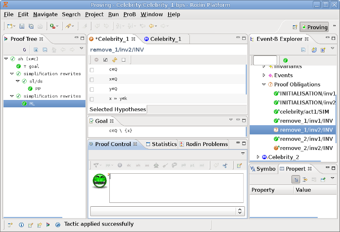
$\includegraphics{img/tutorial/tut_08_proof_final.png}$

Figure 2.21: The green smiley indicates that all sequents of the proof tree are discharged

After saving the proof, the proof obligation remove_1/inv2/INV in the Event-B Explorer should also become a green chop.

$\includegraphics[width=7mm]{img/info_64.png}$
There are alternative ways to prove the proof obligation. For instance, we can use the $\includegraphics[height=2ex]{img/icons/rodin/lasoo_prover.png}$ button to load those hidden hypotheses that contain identifiers in common with the goal into the Selected Hypotheses View, and we can also use it with the selected hypotheses.

In order to move to the next undischarged proof obligation, you may also use the Next Undischarged PO button ( $\includegraphics[height=2ex]{img/icons/rodin/next_prover.png}$ ) of the Proof Control View (3.1.5.4). The next proof can be solved the same way as the last one.

$\includegraphics[width=7mm]{img/info_64.png}$
As an exercise, try to prove Celebrity_2. A small hint: We have to fill in an existential quantifier. First, look in the list of hypothesis to see if you find any variable that is in P and select that hypothesis. Then instantiate b’ and R’ correctly (For instance, if you want to instantiate b’ with c, then $P \backslash \{ c\}$ is a good choice for R’) by typing the instantiations in the Goal View (3.1.5.3) and then clicking on the red existential quantifier. Now all open branches of the proof tree can be proved with p0. After this, we have completed all the proofs, and the model is ready for use.

Footnotes

Interestingly enough, this number can vary: Provers can be configured in the preferences, and changes there can have an impact on the ability to automatically discharge proofs. In addition, all provers have time-outs. On a slow machine, some proof obligations may not get discharged, compared to a faster machine with the same timeout.

Rodin Handbook

2.9.4 The First Proof