Rodin Handbook
This work is sponsored by the Deploy Project
This work is sponsored by the ADVANCE Project
This work is licensed under a Creative Commons Attribution 3.0 Unported License
| Rodin User’s Handbook v.2.8 |
2.10.1 Deadlock Freeness of initial model
Let us look at the initial model which consists of the context doors_ctx1 and the machine doors_0. There are two carrier sets in the model context. One is for people ( ) and the other is for locations (
 ). There is a location called outside (
 ) and a relation (
 ) which defines the places that people are allowed to go. Everyone is permitted to go outside. The model machine has one event, pass, which changes the location of a person and one variable,
  , which denotes where a person is located.
Looking through the initial model, you will see that everything already has been proved (for the initial model and initial contexts). This is true, but Rodin has not yet proved that the model is deadlock free yet, so we will have to prove this ourselves. A model is considered to be deadlocked if the system reaches a state where there are no outgoing transitions. The objective of this section is to develop proofs for deadlock freeness for the initial model and for the first refinement.
Consider the event pass from the initial model:
![\includegraphics[width=7mm]{img/pencil_64.png}](images/img-0005.png)
- EVENTS
- Event
pass

- any
- where

- then

- end
- END


Since the initial model has only one event (pass), the system might deadlock when both guards of the event (grd11 and grd12) are false. In this case, to prove that no deadlocks can occur requires proving that someone can always change room. We must therefore prove that the two guards are always true. To do this, add a new derived invariant (a theorem) to doors_0 called DLF (click once on the label not theorem to make it switch to theorem) and change the predicate so that it is the conjunction of the two guards. The difference between a “normal” invariant and one that is marked as theorem is that you must prove that a theorem is always valid when the previously listed invariants are valid. Then we don’t need to prove that an event preserves the invariant marked as theorem because we can conclude this logically when it already preserves the other invariants.
- INVARIANTS


![\includegraphics[width=7mm]{img/warning_64.png}](images/img-0004.png)
Make sure that when you add your DLF invariant, you add it after the other two invariants in doors_0. The auto prover uses these invariants to prove that the DLF invariant is well defined, and if they aren’t in the right order, the proof obligation DLF/WD will not be discharged
You can also use ProB to search for deadlocks (after ensuring that ProB is installed). Right-click on the machine you want to check and start the animation with the “Start Animation / Model Checking” menu entry. After starting the animation, go to the Event View in the ProB perspective (see Figure 2.9). There are two ways to search for deadlocks:
Press the Check button and mark Find Deadlocks. Then start the model checking by pressing the button Start consistency checking. ProB then systematically “executes” all events and tries to find a state where no event is enabled.
An alternative is to select Deadlock Freedom Checking after clicking on the triangle to the right of the Check button. ProB will then prompt you to input a predicate, but this is optional, so leave it blank. The difference with this alternative alternative is that ProB searches now for variable values where all the invariants are valid but none of the guards are valid.
This contribution requires the ProB plugin. The content is maintained by the plugin contributors and may be out of date.
Save the machine. We see in the Event-B Explorer View that the auto-prover (3.1.7.5) fails to prove the theorem DLF/THM.
If you cannot find the proof obligation DLF/THM, maybe you forgot to mark the invariant as a theorem by clicking once on the not theorem label next to the invariant. Another reason that you might not see the proof obligation DLF/THM is that you have forgotten to rename the invariant “DLF”.
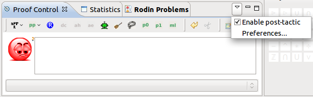
Let us analyze whether this is an inconsistency in the model. Switch to the Proving Perspective and double click on the proof obligation DLF/THM. In the Proof Control view, first disable the post-tactics (there is a small downward pointing arrow in the upper right hand corner above the toolbar (see Figure 2.22). Click on this arrow and make sure that the option Enable post-tactic is unchecked in the dropdown menu.) We are turning off the post-tactics because we want to see the proof develop in its different stages. Now select the root node in the Prove Tree, right-click on it and select Prune. This removes any proof that might be already started by the auto-provers. By doing this we want to assure that you have the same proof as in this tutorial.
In order to succeed with the proof, we need a pair  that is in but not in . Having a look the axioms, we find axm4 of doors_ctx1, which states that there is a location
  different from where everyone is allowed to go:
- AXIOMS


So for every person  in , and
  are in . (In other words: every person is allowed to go to both the outside and a location ). The basic idea of our proof is that a person is either already outside or at the location . If someone is outside, they are allowed to move to , and if they are not outside, they are allowed to move outside. 1.
We assume that there is actually a person, so we need a set that is non-empty. This is automatically the case since carrier sets are always non-empty, but we need a person as an example for our further proof. Now add the hypothesis  by entering this predicate into the Proof Control text area and hitting the
![\includegraphics[height=2ex]{img/icons/rodin/ah_prover.png}](images/img-0341.png) button. In the Proof Tree view you can now see three new nodes have appeared that need to be proven:
button. In the Proof Tree view you can now see three new nodes have appeared that need to be proven:
 is the trivial well-definedness condition. Click on
![\includegraphics[height=2ex]{img/icons/rodin/auto_prover.png}](images/img-0377.png) button to verify it.
button to verify it.  is the hypothesis that we introduced. Click on the
button to verify it.
is the hypothesis that we introduced. Click on the
button to verify it.  is the original goal but we can now use the introduced hypothesis in the proof. We will now continue with the proof of this goal.
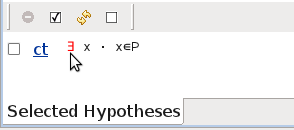
Click on the existential quantifier of the new hypothesis  (appearing in the Selected Hypothesis view) as demonstrated in Figure 2.23. The hypothesis disappears and is replaced by a new hypothesis
  . This is because the value of
  is automatically instantiated. This means that we can use from now on in our proof as an example for a person
If you hover over any red symbol for a short while, a menu will pop up, offering one or more transformations. Make sure that you actually click on the symbol before the menu pops up because otherwise clicking will no longer have any effect. If the menu has popped up before you managed to click on the symbol, you will have to click twice: the first click will discard the menu and the next click will actually perform the operation.
We can prove an existential quantification by giving an example for the variables. First, we instantiate in the goal with the variable that we created: enter in the yellow box corresponding to in the Goal View and click on the existential quantifier as shown in Figure 2.24.
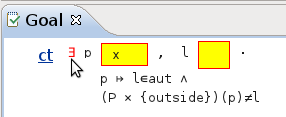 .
.The instantiation produces two new nodes in the Proof Tree view. The first goal is the trivial well-definedness condition and can be easily discharged by pressing
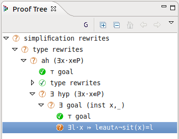
. The remaining goal is  is the result of replacing by in the old goal. You can see the the current proof tree in Figure 2.25. The node with the label ah refers to when we added the hypothesis, the node with the label
  hyp refers to when we instantiated from a hypothesis and the node with the label goal refers to when we instantiated in the goal.
 with .
Now we need an example for the remaining variable . There are two situations we want to distinguish: The person could be outside or not. To distinguish this, type  into the Proof Control view and click on the button
![\includegraphics[height=2ex]{img/icons/rodin/dc_prover.png}](images/img-0387.png) (dc for distinguish case). Again, you get three new goals.
(dc for distinguish case). Again, you get three new goals.
The first is the well-definedness condition of
. must be a function and is in its domain. This is easy to prove since is a total function (3.3.5). Press the
![\includegraphics[height=2ex]{img/icons/rodin/p1.png}](images/img-0388.png) button to verify it.
button to verify it. The second node has the original goal but
as a hypothesis. The third node has the original goal but
 as a hypothesis.
Note that the second and third node will appear identical in the proof tree. You will only see the differences in the hypotheses by selecting the nodes.
Let’s continue with the case  : When is outside, it can always go to the that is defined axm4. To search for axm4, type into the Proof Control text field and click the button
![\includegraphics[height=2ex]{img/icons/rodin/sh_prover.png}](images/img-0346.png) . Add axm4 (
. Add axm4 ( ) to the selected hypotheses. Now click on the red symbol in axm4 (see Figure 2.26) to instantiate . Now we have as an example for a location which is not outside and where everybody can go.
 : The third one is axm4.
 Our goal is still  . Note that the existential quantification introduces a new which does not (yet) have anything to do with the location where anybody can go. Now type into the yellow box of the goal and press the symbol to state that we want to use our as an example for the in the existential quantification. Again, we have the trivial goal as well-definedness condition, so just press
button to verify it. The remaining goal should be
. Note that the existential quantification introduces a new which does not (yet) have anything to do with the location where anybody can go. Now type into the yellow box of the goal and press the symbol to state that we want to use our as an example for the in the existential quantification. Again, we have the trivial goal as well-definedness condition, so just press
button to verify it. The remaining goal should be  . This can be proven with the selected hypotheses ,
  and
and  . Press the
button to verify this goal.
. Press the
button to verify this goal.
Now only second case of the case distinction remains. This is where is not outside ( ). In this case, can simply go outside. Again the goal is . Type as an example for a location into the yellow box and press the symbol. Press the
button to discharge the trivial well-definedness condition . The new goal should be
). In this case, can simply go outside. Again the goal is . Type as an example for a location into the yellow box and press the symbol. Press the
button to discharge the trivial well-definedness condition . The new goal should be  .
.
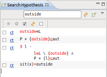
To prove this we need to prove that has the right to go . This is stated in the axiom  . Have a look at the Search Hypothesis view. This was also one of the results from the last search for . (If you no longer see the results, repeat the search by entering into the Proof Control and press the
button.) Select (in Figure 2.26, it’s the second entry) and press the
. Have a look at the Search Hypothesis view. This was also one of the results from the last search for . (If you no longer see the results, repeat the search by entering into the Proof Control and press the
button.) Select (in Figure 2.26, it’s the second entry) and press the
![\includegraphics[height=2ex]{img/icons/rodin/add.png}](images/img-0347.png) button to add it to your selected hypothesis. The auto-prover now has enough hypotheses, so simply click the
button and the last goal of our theorem should be proven.
button to add it to your selected hypothesis. The auto-prover now has enough hypotheses, so simply click the
button and the last goal of our theorem should be proven.
Here is the summary of the proof. Compare this with your final proof tree (as shown in Figure 2.27).
added hypotheses: |
well-definedness condition |
the hypotheses: automatically proven |
instantiation of |
using |
well-definedness condition |
case distinction |
well-definedness condition ( |
domain): proven using the p1 provers |
first case: instantiation of |
using |
well-definedness condition |
remaining goal: automatically proven |
second case: using |
for the |
well-definedness condition |
hypotheses |
remaining goal: automatically proven |
 in the goal
 in the goal
 selected
 : The third one is axm4.
Footnotes
- One could argue that this is too restrictive in the real world: After all, why do all people need authorisation for the same location l? But arguing about the realism of the example is out of the scope.